About Sales Trends and Forecast
Sales Trends and Forecast is an Odoo tool that lets you generate sales reports by period and apply statistical methods to scientifically forecast further periods.
The app assumes applying statistical methods to calculate historical sales trends and make a forecast. Experiment with different statistical models and parameters to ensure the most reliable prognosis, taking advantage of the proven methods offered by statsmodels.
The tool introduces a special user-friendly interface that allows you to instantly calculate sales series. Easily switch between various reports and adjust settings with just a few clicks. Additionally, analyze data in pivot, graph, or chart views for full control over your sales data. Export series as Excel tables for further analysis or reporting.
Shrink considered order/quotation lines flexibly or analyze the overall sales performance of your company. Group your data into different series for more detailed analysis and insights.
Apply time frames for historical data and focus on intervals that are relevant to your industry. This flexibility allows you to adapt the tool to your specific needs. Additionally, you can seamlessly work with both past and future periods, ensuring you have a comprehensive understanding of your sales trends and forecasts.
Scientific Approach to Forecasting
Focused Analysis
Innovative Data Analysis Interface
Topical Data
Forecast Report and Historical Data
A forecast report is a report that helps to analyze historical data. It provides businesses with valuable information about future sales trends and patterns. Forecast reports help businesses make informed decisions regarding inventory management, resource allocation, production planning, and overall financial management. For example, with the help of the sales forecast report, businesses can align their marketing efforts, pricing strategies, and advertising campaigns to maximize sales potential.
The app allows users to create multiple sales forecast reports to compare the results and refer to them for further decision-making. This way, you can find the best approach to create a forecast report that corresponds to the business peculiarities and is just more accurate.
The forecast report is generated based on the actual Odoo sales data, in particular, it works with quotations and sales orders (models sale.order and sale.order.line) and their fields. For that, the app extracts data from the standard Odoo sales report table (model sale.report, see menu Sales > Reporting), where the sales data is grouped and aggregated in a single currency by default.
The report relies on the following fields:
1. Customer: The customer information is sourced from the 'Customer' field on the order. Using this field, the module can extract additional information about the customer's country and industry from the 'Country' and 'Industry' fields of the contact object.
2. Product in each sale line: The module analyzes each sale line and includes information about the product, such as the related product template. The category information is obtained from the 'Product Category' field. Additionally, the volume and gross weight of the product are extracted from the 'Volume' and 'Weight' fields.
3. Total fields: The sale order's total amount and the untaxed total, is obtained from the 'Total' and 'Untaxed amount' fields of the sale order. Based on the field 'Invoiced' by each product line of the sale order, the module retrieves the information on the untaxed amount to invoice and the untaxed amount invoiced.
4. Sales team: The sales team's information is obtained from the sales order 'Sales Team' field.
5. Salesperson: The salesperson's information is extracted from the 'Salesperson' field.
6. Order date: The creation date of the sale order is retrieved from the 'Order date' field.
7. State: The state of the sale order is obtained from the 'State' field (see above the sale order form).
8. Company: The company's information is sourced from the sales order 'Company' field.
For example, take a look at the quotation form, where, in particular, the following fields are visible: salesperson, sales team, company, customer, product, state, total, untaxed amount, invoiced, and order date.
Once the data from the sale order fields is extracted, it can be further manipulated by filtering, grouping, and analyzing it.
Please, take into account, that different users may have different access to the sale orders. As a result, different data may be extracted from the database. Therefore, the sales forecast report may look different for different users (see Access rights).
The basis of the sales forecast report depends on the specific requirements and analysis needs of the business. As a basic measurement for the sales forecast report, you can use the following:
1. Sales Total (in the default company currency). It provides the total amount of sales revenue generated within a specific period. It gives an overview of the overall sales performance without considering any taxes or other factors.
2. Untaxed Total (in the default company currency). It excludes any taxes from the sales amount and provides a more accurate representation of the revenue earned from the sale of products, or services.
3. Untaxed Amount to Invoice (in the default company currency). It considers the sales that are yet to be invoiced. It provides an estimate of the potential revenue the business can expect to generate based on pending invoices.
4. Untaxed Amount Invoiced (in the default company currency). It considers the sales that are already invoiced. It may provide a clearer result, while the pending, or canceled invoices aren't taken into consideration to predict the revenue.
5. Gross Weight. It analyzes the sales forecast based on the weight of the products sold. It can be useful for businesses dealing with physical goods that have weight-based pricing or shipping considerations.
6. Volume. It focuses on the volume of products sold, providing insights into the sales forecast based on the number of items and their size sold rather than the monetary value.
You can choose the basis for the forecast in the section 'Parameter' in the left part of the interface.
With the help of filters, that are based on the sale order fields, users can further limit the data that should be used in the forecast. This can help identify specific patterns or trends related to the factors of interest. Additionally, the filters can be applied iteratively, allowing users to experiment with different scenarios and evaluate their impact on the sales forecasts.
To apply filters to the sale data, users can choose one or multiple options from the related fields in the "Filters" section on the left side of the interface. You can apply filters by:
1. Product category: Narrow down the analysis to a specific product category or categories. For example, you can forecast sales for 'Office Furniture' only, or for both 'Office Furniture' and 'Services'. Filtering is based on the 'Product Category' field, which can be found on the sale order lines on the sale order form.
2. Product template: Refine the analysis by selecting specific product templates. For instance, you can forecast sales for the 'Customizable desk' template, or for both the 'Customizable desk' and 'Chair' templates. The module utilizes the product's details available through the sale order lines.
3. Product variant: Focus the analysis on particular product variants. For example, you can forecast sales for the 'White aluminum desk' variant, or for both the 'White aluminum desk' and 'Black steel desk' variants. Filtering is based on the product's details accessed through the sale order lines of a linked quotation.
4. Company: Limit the analysis to specific companies. For instance, you can forecast sales for the 'Chicago' company, or for both the 'San Francisco' and 'Chicago' companies. The module relies on the 'Company' field of a sale order.
5. Sales team: Narrow down the analysis to specific sales teams. For example, you can forecast sales for the 'America' sales team, or for both the 'America' and 'Europe' sales teams. Filtering is based on the 'Sales team' field.
6. Salesperson: Filter the analysis by specific salespersons. For instance, you can forecast sales for 'Anita Oliver', or for both 'Anita Oliver' and 'Abigail Peterson'. Filtering is based on the 'Salesperson' field.
7. Country: Refine the analysis by selecting specific countries. For example, you can forecast sales in the US, or in both the US and Belgium. The module relies on the 'Company' field of a related contact, which can be accessed through the 'Customer' field on the sale order form.
8. Industry: Narrow down the analysis to specific industries. For example, you can forecast sales for customers from the Construction industry, or for both the Construction and Agriculture industries. Filtering is based on the 'Industry' field of a linked partner.
9. Customer: Limit the analysis to specific customers. For example, you can forecast sales for the regular customer 'Azure Interior', or for both 'Azure Interior' and 'Deco Addict'. The module relies on the 'Customer' field.
As you limit the data with the help of filters, you can choose one, or several options per each filter field. When you choose several options in the same filtering field, then the sale orders that have ANY of the options are considered for the forecast. For example, you can forecast sales for the products in two categories 'Office Furniture' and 'Services', then the sale orders that contain products from the category 'Office Furniture' and the sale orders that contain products from the category 'Services' will be taken into consideration.
When you choose options in different filter fields, then the sale orders that match ALL the criteria are considered for the forecast. For example, you can specify filters by product categories 'Office furniture' and 'Services', particular country 'the US', and the sales team 'America'. This way, you would narrow down the dataset to only include sale orders that meet all three criteria. This would allow you to analyze sales trends and patterns specific to the categories 'Office Furniture' and 'Services', within the United States market, and under the sales team America.
Another option to further refine the historical data used for forecasting, is through filtering sales orders by their states. The available states are Sales Done, Sales Order, Quotation Sent, Draft Quotation, and Cancelled. By selecting only the relevant states, such as Sales Done and Sales Order, you can exclude canceled or draft sales orders that may provide confusing or irrelevant information for the forecast.
In the interface, you can find the 'States' section in the left part of the interface. Tick the required states to choose which sale orders should be included in the forecast report. By excluding the canceled sale orders, for example, you can focus on the sales that are most likely to contribute to future sales and disregard any potential outliers.
You can choose multiple sale order states, then only the sale orders in the selected states will be considered for the forecast.
In case the existing filters by sale data and states aren't enough, you can also add your own filters by any sale report column. This way, you can flexibly limit the historical data that is used to forecast sales.
For that, in the section 'Extra Filters', click 'Add a line', choose the field by scrolling or typing the beginning in the search field, and choose the filter options. For example, you can create a filter 'Total is >= 10000' to consider only the sales orders with the total more or equal to 10000.
You can also add a complex filter with one, or several conditions. For that, click on the '+' icon on the right side of the rule you wrote and, in the new line add a new filter option. After that, you will see the ANY or ALL button above, so only documents that match ANY of the rules or ALL rules will be shown. For example, consider only the sales orders with a total of more or equal to 10000 with the invoice status 'To invoice' by adding 2 filters 'Total is >= 10000' and 'Invoice Status = To Invoice', and choosing the option 'All' above.
You can further narrow down the historical data by specifying the time frame. The module allows specifying the start/end date to limit the historical data, choosing the type of period to group the historical data, and specifying the number of periods you want to forecast. The module relies on the field 'Order date' of a linked quotation to define to what period a sale order refers to and whether it should be considered for the forecast, or not.
You can limit the historical data by specifying the period start/end date. In this case, if the order date of a sale order is within the period, then it will be used as historical data for the forecast. For example, if you specify the start and end date as 01/01/2023 - 31/12/2023, then only the sale orders created during the year 2023 will be used as the historical data for the forecast.
As you specify the type (length) of the period, the module groups and summarizes the sale orders with the order date within each period. The period's length can be in days, weeks, months, quarters, or even years. It is only up to you which period type to choose depending on available data, your specific requirements, and business needs. For example, if you are in the retail industry, you can split your sales data by month to identify the months with the highest and lowest sales figures. This can help you optimize your inventory and marketing strategies accordingly. Similarly, in the tourism industry, you can split your data by quarters to understand seasonal trends and plan promotional campaigns or discounts during low seasons.
When you set the number of forecasted periods, you define what should be forecasted. This way, based on the chosen end date, the module generates a forecast for the next N periods. In case, the field end date is left empty, then the module generates a forecast for the next N periods, including the current one. For example, if you set the start and end date as 01/01/2023 - 31/12/2023, choose the period type as 'Monthly', and set the number of forecasted periods as 2, then the module will generate the forecast for January and February 2024. If the end date wasn't specified and now it is 13 February 2024, then the module will generate a forecast for February and March 2024.
Statistical Models
The app assumes applying statistical methods to calculate historical sales trends and make a forecast. A stats model is a mathematical model with the set parameters that is used to create a sales forecast based on the available historical data. It is used to describe the relationship between variables in a dataset and make future predictions.
Stats models have different complexity, and their own unique parameters, and might be suitable for a definite market or a specific business. Models help to understand the underlying patterns, relationships, and variability in data, and aid in making statistical inferences and predictions.
The following stats models are used by the module to predict future sales:
1. Autoregression (AR)
2. Autoregressive Distributed Lag (ARDR)
3. Autoregressive Integrated Moving Average (ARIMA)
4. Seasonal Autoregressive Integrated Moving Average (SARIMAX)
5. Simple Exponential Smoothing (SES)
6. Holt Winter's Exponential Smoothing (HWES) (see The List of Models).
Before generating a sales forecast, it is necessary to create one, or several stats models. Creating a model allows configuring the parameters related to the chosen stats model. Users have the flexibility to choose between using preset parameters or implementing advanced settings, thereby catering to the needs of both seasoned statisticians and beginners in the field.
To create a stats model for the forecast:
1. Open the Sales app
2. In the systray, go to Trends&Forecast > Stats Models
3. Click 'New'
4. Choose the forecasting method
5. Write the reference
6. Depending on the chosen model, the list of parameters in the tab 'Parameters' will change. Optionally, configure the existing parameters. Hover over the field's titles to get the help hints.
7. Open the tab 'Help' and look through the articles, for deep details about what each stats model means and which parameters might be applied.
The List of Models
Here you will find the description of the stats models that are used by the module.
Autoregression (AR)
In an autoregression model, the sales today are expressed as a linear combination of the sales from previous periods, with some unpredictable noise added. The model does not take into account any seasonal effects, purely defined trends, or abnormal observations that need to be smoothed out. However, despite these limitations, autoregression models are highly versatile and can effectively capture nearly any autocorrelation pattern. They serve as a universal model for autocorrelation in time series data.
Autoregression models can be useful for short-term sales forecasting or predicting any other time-dependent variable based on its past values. By analyzing the autocorrelation within the data, the model can identify patterns and use them to make predictions about future values.
Autoregressive Distributed Lag (ARDR)
The Autoregressive Distributed Lag (ARDL) model is commonly used in econometrics to analyze the relationship between a dependent variable and a set of independent variables over a period of time. Unlike the standard autoregressive models that only consider the past values of the dependent variable, the ARDL model incorporates the past values of other relevant time series as well.
By including lagged values of both the dependent variable and other relevant time series, the ARDL model captures both short-term dynamics and long-run relationships. This makes it particularly useful for forecasting long-term trends based on the short-term dynamics observed in the data. The estimation of the ARDL model involves determining the appropriate lag lengths for both the dependent variable and other time series.
Autoregressive Integrated Moving Average (ARIMA)
ARIMA is a versatile and widely used forecasting model that is capable of capturing a range of temporal patterns in time series data. It combines three components:
1. Autoregressive (AR): This component uses past values of the time series itself to predict future values. It assumes that the future value of a series is linearly dependent on its past values.
2. Integrated (I): The integration component is employed to transform non-stationary data into stationary data. Stationarity means that the statistical properties of the data, such as mean and variance, do not change over time. By differencing the time series, ARIMA can eliminate trends and make the data stationary.
3. Moving Average (MA): This component utilizes the errors or residuals from past forecasts to predict future values. It assumes that the future value of a series is related to the average of the past forecast errors.
A key requirement for using ARIMA is that the data should be collected at fixed intervals, such as monthly, quarterly, or yearly. This ensures that the model can capture the time dependence and make meaningful predictions. ARIMA is particularly useful for nonseasonal data, where the patterns are not tied to specific periods.
Seasonal Autoregressive Integrated Moving-Average (SARIMAX)
SARIMAX combines the regular ARIMA model with additional parameters that capture seasonal patterns. This allows the model to account for the seasonal variations in the data and make more accurate predictions.
By including the seasonal components, SARIMAX can capture long-term trends as well as short-term cycles in the data. This makes it a powerful tool for modeling and forecasting time series data that exhibit seasonality.
SARIMAX models can be estimated using various techniques, such as maximum likelihood estimation. Once the model is fitted to the historical data, it can be used to forecast future values.
Simple Exponential Smoothing (SES)
Simple Exponential Smoothing (SES) is a time series forecasting method that is used to predict future values based on historical data. It is a basic form of exponential smoothing, commonly employed when there are no significant trends or seasonal patterns in the data.
In SES, each forecast value is determined by the weighted average of past observations, with more recent observations given higher weights. The model assigns exponentially decreasing weights to the previous data points, which ensures that older observations have limited influence on the forecasts. This characteristic of SES makes it particularly useful for short-term forecasting.
While SES is a relatively simple model, it does not consider any external factors that may affect the data, such as trends or seasonal patterns. This limitation can lead to inaccurate forecasts in cases where such patterns exist in the data. To address this limitation, a variant of SES called Seasonal Exponential Smoothing (also known as Holt-Winters Method) is employed. By considering seasonal patterns, SES becomes more powerful in making accurate forecasts for data that exhibit repeating patterns, such as sales data with monthly or quarterly cycles.
Holt Winter's Exponential Smoothing (HWES)
Holt Winter's Exponential Smoothing (HWES) is a time-series forecasting method that uses exponential smoothing to make predictions based on past observations. The method considers three components of a time series: level, trend, and seasonality, and uses them to make forecasts for future periods. It enriches the SES method to work with time series trends and seasonal effects. The model can provide more accurate forecasts for longer-term periods.
The level component represents the average value of the time series, and it is updated at each period based on the latest observation. The trend component captures any upward or downward movement in the time series over time, and it is updated based on the difference between the current level and the previous level. The seasonality component represents any regular pattern or cycle that occurs in the time series, such as monthly or yearly fluctuations.
HWES uses separate smoothing parameters for each of these components to adjust the weights given to the observations. This flexibility allows it to adapt to different types of time series data and capture their unique characteristics.
To make forecasts using HWES, the method uses a combination of the latest level, trend, and seasonality values to project future values. The weights assigned to the components depend on the chosen smoothing parameters. By adjusting these parameters, analysts can control the balance between the importance of recent observations and the overall trend and seasonality patterns.
Choosing a Model for Forecast
The app provides a statistical methods of different complexity that you can experiment with to retrieve trends. It is important to note that there is no one-size-fits-all approach and the suitability of different methods can vary depending on various factors such as the market, industry, firm, circumstances, and quality of historical data.
It is possible that certain models with specific parameters may not make accurate predictions or may provide unrealistic results. Therefore, it is essential to carefully analyze and evaluate the outcomes of different methods.
To get accurate predictions, it is necessary to experiment with different statistical models and adjust the parameters accordingly. The app provides the functionality to compare the forecasted data with the actual values to evaluate the effectiveness of the chosen models.
To verify a specific assumption using historical data, you can make predictions for past periods. For that, while creating a forecast report, find the section 'Extra Settings' and tick the option 'Hypothesis Testing'. For example, if you have sales orders from 2017 to 2022, you can generate a report using historical data for the period of 2017-2021 and forecast the 12 months of 2022. This allows you to obtain predictions for a time frame for which you already have actual values. Therefore, by comparing the forecasted and actual values, you can assess the accuracy and suitability of the selected model and factors.
By using the app, you can save time and effort by quickly comparing multiple statistical models and their corresponding hypotheses. To compare and analyze multiple statistical models simultaneously, add them to the field 'Stats Models' while creating a report. This way, you can determine the most appropriate model or decide whether further experimentation is required to improve the predictions
When creating a sales forecast report, sometimes, it might be essential to consider the seasonal changes that might impact the business. Seasonal changes refer to the fluctuation in customer demand and sales due to factors like holidays, weather conditions, or cultural events that occur at specific times of the year. Taking into account these peculiarities can significantly improve the accuracy and reliability of the sales forecast. For example, a retailer might stock up on decorative items before the holiday season to meet the increased demand during that time and avoid overstocking those during the times, when the demand is low.
To consider the seasonal changes while creating a sales forecast, choose the statistical models that imply that, for example, SARIMAX, or HWES (see The List of Models).
Usage Requirements
To effectively use the app and reveal trends, it is necessary to have a sufficient amount of historical data. For example, it is hardly possible to generate an accurate sales report for the next month, based on the three previous ones.
At the same time, simply having a large amount of sales data is not enough if it lacks meaningful trends and insights. For example, we have a clothing company with a vast amount of sales data from the previous year, including various products, and geographic regions. Without actual trends derived from the sales data, the company may mistakenly assume that all products and regions will experience equal sales growth during the holiday season. However, the actual increase in sales may relate to winter clothing, party outfits, and festive accessories. They may also discover that customers in a specific region tend to spend more during the holidays compared to others.
To get accurate predictions, it is typically necessary to extensively experiment with various statistical models and the introduced parameters. This process allows configuring the models and optimizing their performance. For example, it may be useful to create a forecast report for multiple stats models at once or generate a report for the past periods with the help of 'Hypothesis Testing' (see Choosing a Model for Forecast).
To use the full capabilities of the app, it is also recommended to have at least a basic understanding of statistics. This knowledge will enable users to interpret the output effectively and make informed decisions based on the predictions generated by the app.
Useful Links
The app was inspired by a number of articles that provide a detailed description of the stats models and the way they are implemented. The articles outlined the nuances of different statistical techniques and the algorithms used in building these models.
You can refer to these articles, to get deeper insights into various statistical methods and guidance on how to implement them effectively:
1. 11 Classical Time Series Forecasting Methods in Python (Cheat Sheet)
2. A Guide to Time Series Forecasting with ARIMA in Python 3
3. ARIMA models for time series forecasting
You can also refer to any other articles regarding the methods used in the module, while the module is based on the universal statistical methods.
Forecast Creation & Interface
The module provides a user-friendly and flexible way to analyze and forecast sales through the special interface, making it easier for businesses to make informed decisions and plan for the future. There, you can flexibly switch between different reports and update settings in just a few clicks. To find the module's interface:
1. Open the 'Sales' app
2. In the systray, find the button 'Trends&Forecast' and choose the option 'Analysis'.
The interface consists of two parts, the domain constructor on the left and the result of the forecast on the right.
The appearance of the resulting table may be different depending on the configurations applied. You can compare the forecasted result of multiple stats models in the same table, split data series in various periods assumed in your industry or business area, introduce a few data series simultaneously with the help of grouping, check hypotheses, visualize the result with the help of graph views, refer to the basic statistical info, and shorten figures for the best result. Additionally, users can conveniently export the table for future reference.
Forecast Creation
The sales forecast constructor is a user-friendly tool that helps customize and improve sales predictions. It's conveniently located on the left side of the interface. Users can easily modify input parameters to fit their needs. They can choose the number of forecast periods, select statistical models, analyze specific parameters, and apply filters to narrow down outputs. This feature improves prediction accuracy and aids decision-making.
For instance, imagine a retail manager preparing for the holiday season. With the sales forecast constructor, they can easily manipulate parameters to forecast sales for the next three months. They can choose a robust statistical model based on past trends and focus on the product type with the highest demand. Filters can be applied to consider only relevant sales channels. By using these tools, the manager can accurately forecast sales and make informed decisions about inventory, staffing, and promotions.
To create a new sales forecast:
1. As you open the 'Trends&Forecast' > 'Analysis' submenu, in the left functional interface, choose the option '…new'.
2. Choose a type of period in the section 'Historical data'.
This way, you specify the periodicity with which the data series should be split in the table. The available options are Daily, Weekly, Monthly, Quarterly, and Yearly.
For example, choose the option 'Monthly'. Then, in the resulting table, you will see the following lines: October 2023, November 2023, December 2023, etc.
3. Below, in the fields 'period start' and 'period end' choose the dates.
This will give the instructions to the module on what historical data to take into consideration while generating a sales forecast. For example, set the period start as 01.01.2023, and the period end as 31.12.2023 to consider the historical data for the year 2023.
It is possible to leave the fields empty to consider all available historical data.
4. In the section 'Stats Models' choose the statistical models for the forecast.
You can apply as many, and as different statistical models as you want to check. Based on the chosen model the result can be different.
In order to make a statistical model available for selection in the field, you should create it first (see Statistical Models).
For example, to consider seasonal patterns in the data, create and choose the stats models SARIMAX and HWES and compare the result (see The List of Models).
5. In the section 'Forecast Periods' choose the number of periods to forecast.
This way, you specify how many periods should be forecasted. You can choose an unlimited number of periods to predict future periods or check hypotheses.
For example, if you choose the type of period as a month (step 2) and set the forecast periods as 3, then the app will generate a prediction for the next 3 months.
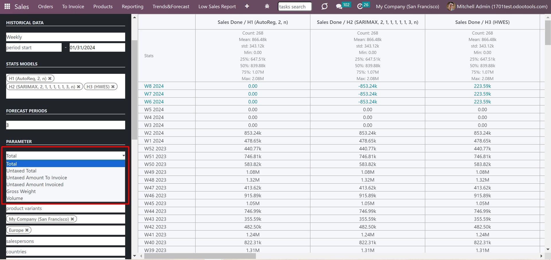
6. Choose the parameter to analyze.
The parameters serve as a basis for the forecast. The available parameters are a sales total, an untaxed total, an untaxed total to invoice, gross weight, or volume (see Forecast Report and Historical Data).
For example, choose the parameter sales total, to consider the total amount of sales revenue as a base for the forecast. It would give an overview of the overall sales performance without considering any taxes or other factors.
7. In the section 'Filters', choose the filters to limit the sales data.
It is possible to limit the sales data by product categories, product templates, product variants, sales teams, salespersons, countries, industries, and specific customers.
For example, you can limit the sales data to only include product categories such as 'All/Consumable' or 'All/Saleable'. This would allow you to focus on specific types of products within your sales analysis.
In case you work in a multi-company regime, you can also choose the company in the filtering field 'Companies' to consider only related records for the forecast.
In case the available filters aren't enough, you can also create your own criteria based on Odoo's dynamic domain constructor in the section 'Extra Filters. This allows you to define criteria based on any sale line storable fields, giving you complete flexibility in analyzing your sales data.
8. In the section 'States', tick the states of the sale orders that should be taken into consideration to make a forecast.
The available states are: Sales Done, Sales Order, Quotation Sent, Draft Quotation, and Cancelled.
For example, if you want to consider only the completed and confirmed sale orders, you can choose the states 'Sales Done' and 'Sales Order' to make a forecast.
9. In the section 'Group By', choose the grouping criteria that will be applied to the forecast table.
It is possible to group by a product category, a product template, a product variant, an order state, a team, a salesperson, a country, an industry, a customer, or a company. This way, you can introduce a few data series simultaneously.
For example, group the forecast by the order state to compare the sales performance of different order states.
10. Tick the option 'Show Stats Info' to show the general statistical measurement of the series.
If ticked, then in the first row of the table you will see the basic statistical info: count, mean, standard deviation, minimum, maximum, 25%, 50%, and 75% factors.
For example, you can find out the total number of records that are considered for the forecast by referring to the line 'Count'.
11. Tick the option 'Hypothesis Testing' to compare predicted values to real historical data if any (see Hypothesis Testing).
To verify a specific assumption using historical data, you can make predictions for past periods. This way, if the historical data exists for the predicted period, it will be written below the forecasted value. This way you can compare the values and choose the stats model that suits the best.
For example, if you have sales orders from 2017 to 2022, you can generate a report using historical data for the period of 2017-2021 and forecast the 12 months of 2022. Then, the stats model with the closest values might be the best option to forecast sales for further periods.
12. Tick the option 'Shorten Figures' to make figures human-readable, otherwise, they will be shown precisely.
It might be more convenient to work with rounded figures when the sales number is in thousands or millions. For example, it may be more convenient to refer to the number 200k than 192,217.
Even after generating a table with rounded figures, you can see the precise number by hovering over a certain figure.
13. Click 'Refresh' to apply the parameters and see the result on the right side.
14. Click 'Save', introduce the name of the report, and then click 'Save&Close' to save the sales forecast report.
After generating and saving a sales trends record, you have the flexibility to explore different scenarios without having to start over. By making adjustments to the forecast, you can instantly see the impact without the need to save it.
To make changes to the forecast, simply introduce the changes and click on the 'Refresh' button. The result will be immediately updated in the table on the right side of the interface. You can repeat this process multiple times, refining your forecast until you are satisfied with the outcome. If you wish to save the modified forecast, you have the option to create a new report or update an existing one. This enables you to maintain a record of your forecasting experiments for future reference.
Only users with the 'Sales Forecast' right and access to the 'Sales' app can view and manage sales forecast reports (see Access Rights).

Result Appearance
When analyzing data and making predictions, having a clear and organized representation of the results is crucial. Different configurations and options may influence the appearance of the resulting table, providing flexibility and customization. You can compare the forecasted result of multiple stats models in the same table, split data series in various periods assumed in your industry or business area, introduce a few data series simultaneously with the help of grouping, check hypotheses, visualize the result with the help of graph views, refer to the basic statistical info, and shorten figures for the best result. Additionally, users can conveniently export the table for future reference.
The module provides a convenient way to access the key statistical measurements of a series, conveniently displayed in the first row of the table. To access these statistics, simply enable the 'Show Stats Info' option located at the end of the left part of the user interface. Once enabled, a separate row dedicated to statistics will be added to the table. This row will present a comprehensive set of information including the Count, Mean, Standard Deviation, Minimum, and Maximum, as well as the 25%, 50%, and 75% factors.
The module provides visual representations of forecasted data, including charts and graphs, to enhance understanding and analysis of trends. Users can easily switch between table, chart, and graph views using the buttons located at the top of the left-side interface.
To access the line chart, click on the second icon. The vertical scale displays sales figures, while the horizontal scale represents dates. The curve on the chart highlights both historical and forecasted values, denoted by small dots. By hovering over any dot on the curve, users can obtain specific details such as the corresponding period, stats model, and exact value.
If grouping is applied, each distinct group will be presented as a separate curve with its color and set of values. All available grouping options, distinguished by colors, are displayed above the chart. Users can conveniently show or hide specific groups from the chart by clicking on the corresponding grouping option.
To switch to the graph chart, click on the third icon. Similar to the line chart, sales numbers are depicted on the vertical scale and dates on the horizontal scale. Historical and forecasted values are represented by the vertical lines on the graph. Hovering over a line reveals detailed information such as the corresponding period, stats model, and precise value.
When grouping is applied, each group is color-coded and positioned alongside each other on the respective period. All available grouping options, distinguished by colors, are displayed above the graph. Users can conveniently show or hide specific groups from the graph by clicking on the corresponding grouping option.
You can easily export the resulting table for future reference. To do this, select the existing report from the selector, or configure a new one, and click on the 'Export' button. Then, the downloading of the .xlsx file will start immediately.
In the exported table, just like in the one in Odoo, the predicted periods will be indicated in blue color, while periods with historical data will be marked in black. The periods are presented on the vertical scale, with the models and grouping criteria shown on the horizontal scale.
The selection of statistical models and grouping options greatly impacts the structure of the resulting table.
With the help of grouping, multiple data series can be presented simultaneously. Each grouping option is displayed as a separate column in the table, enabling easy comparison and further analysis. Various grouping options such as product category, template, variant, order state, team, salesperson, country, industry, customer, or company can be applied. For instance, by grouping by sales team, you can examine the forecast for each team individually.
Alternatively, you have the option to generate a general forecast without applying any grouping. This allows you to view the overall result.
To generate a forecast, you can choose a single model, which you find the most relevant and it will be displayed on the vertical scale of the table. Alternatively, if you aren't sure which stats model is the best in your case, you can select several ones and show them in the same table. In this case, each model will be represented by its column in the resulting table. Each model will evaluate its specific data series and provide predictions accordingly. For example, if a company wishes to consider seasonal changes, it can select models such as SARIMAX and HWES to include predictions from both. The table will then include two columns with the forecast, one for the SARIMAX model and one for the HWES model.
When multiple models are chosen and a grouping option is applied, a separate column is added for each stats model with a grouping option. This is especially useful when there is a need to compare the forecast for different data series, within a single table. For example, we have selected two stats models SARIMAX and HWES, and applied the grouping by sales teams (America, Europe). In the resulting table, the following columns were added: SARIMAX America, SARIMAX Europe, HWES America, and HWES Europe.
To verify a specific assumption using historical data, you can make predictions for past periods. Then, if the historical data exists for the predicted period, it will be written below the forecasted value. This way, you can compare the values and choose the stats model that suits the best. For example, if you have sales orders from 2017 to 2022, you can generate a report using historical data for the period of 2017-2021 and forecast the 12 months of 2022. Then, the stats model with the closest values might be the best option to forecast sales for further periods (see Choosing a Model for Forecast).

For extra convenience, you can work with the numbers rounded in thousands, or millions. This would make the figures human readable. For example, it may be more convenient to refer to the number 200k than 192,217.
Even with rounded figures in the table, you can still see the precise numbers by hovering over a particular figure. For example, the number 3248380 will be shown as 3.25M, but as you hover over it, you will see the full number 3248380.
Access Rights
The right to access the module's features belongs to the users with the group Sales > Sales Forecast assigned. You can grant the right to forecast tools for any salesperson if you want a user to be able to see and manage sales forecast reports. If a salesperson doesn't have the role assigned, the related menu will be hidden for him/her.
To assign the user group to one or several users:
1. Go to General Settings
2. Click 'Manage Users' and choose a user
3. Find the section 'Sales' and in the field 'Sales Forecast' choose the option 'Sales Forecast'.
After that, the user will see the option 'Trends&Forecast' in the systray of the Sales app.
The appearance of the sales forecast report's table may vary depending on the user's access rights. The report takes into consideration the available companies and sale orders that the user has access to. This ensures that the user sees only the data relevant to their access level.
For instance, if a user has access to the 'San Francisco' company but not the 'Chicago' company, the resulting table will display the historical data and forecast specifically for the 'San Francisco' company.
Moreover, the sales forecast report will only include the sale orders that a user has access to. This means that only the historical data that the user can access will be used for forecasting sales.
For example, let's consider Anita Oliver who has the sales role 'Only own' assigned. In this scenario, the sales forecast table will display historical data and forecasted data solely based on her own sale orders, regardless of any filters that may be set.
About Sales Trends and Forecast
Sales Trends and Forecast is an Odoo tool that lets you generate sales reports by period and apply statistical methods to scientifically forecast further periods.
The app assumes applying statistical methods to calculate historical sales trends and make a forecast. Experiment with different statistical models and parameters to ensure the most reliable prognosis, taking advantage of the proven methods offered by statsmodels.
The tool introduces a special user-friendly interface that allows you to instantly calculate sales series. Easily switch between various reports and adjust settings with just a few clicks. Additionally, analyze data in pivot, graph, or chart views for full control over your sales data. Export series as Excel tables for further analysis or reporting.
Shrink considered order/quotation lines flexibly or analyze the overall sales performance of your company. Group your data into different series for more detailed analysis and insights.
Apply time frames for historical data and focus on intervals that are relevant to your industry. This flexibility allows you to adapt the tool to your specific needs. Additionally, you can seamlessly work with both past and future periods, ensuring you have a comprehensive understanding of your sales trends and forecasts.
Scientific Approach to Forecasting
Focused Analysis
Innovative Data Analysis Interface
Topical Data
Forecast Report and Historical Data
A forecast report is a report that helps to analyze historical data. It provides businesses with valuable information about future sales trends and patterns. Forecast reports help businesses make informed decisions regarding inventory management, resource allocation, production planning, and overall financial management. For example, with the help of the sales forecast report, businesses can align their marketing efforts, pricing strategies, and advertising campaigns to maximize sales potential.
The app allows users to create multiple sales forecast reports to compare the results and refer to them for further decision-making. This way, you can find the best approach to create a forecast report that corresponds to the business peculiarities and is just more accurate.
The forecast report is generated based on the actual Odoo sales data, in particular, it works with quotations and sales orders (models sale.order and sale.order.line) and their fields. For that, the app extracts data from the standard Odoo sales report table (model sale.report, see menu Sales > Reporting), where the sales data is grouped and aggregated in a single currency by default.
The report relies on the following fields:
1. Customer: The customer information is sourced from the 'Customer' field on the order. Using this field, the module can extract additional information about the customer's country and industry from the 'Country' and 'Industry' fields of the contact object.
2. Product in each sale line: The module analyzes each sale line and includes information about the product, such as the related product template. The category information is obtained from the 'Product Category' field. Additionally, the volume and gross weight of the product are extracted from the 'Volume' and 'Weight' fields.
3. Total fields: The sale order's total amount and the untaxed total, is obtained from the 'Total' and 'Untaxed amount' fields of the sale order. Based on the field 'Invoiced' by each product line of the sale order, the module retrieves the information on the untaxed amount to invoice and the untaxed amount invoiced.
4. Sales team: The sales team's information is obtained from the sales order 'Sales Team' field.
5. Salesperson: The salesperson's information is extracted from the 'Salesperson' field.
6. Order date: The creation date of the sale order is retrieved from the 'Order date' field.
7. State: The state of the sale order is obtained from the 'State' field (see above the sale order form).
8. Company: The company's information is sourced from the sales order 'Company' field.
For example, take a look at the quotation form, where, in particular, the following fields are visible: salesperson, sales team, company, customer, product, state, total, untaxed amount, invoiced, and order date.
Once the data from the sale order fields is extracted, it can be further manipulated by filtering, grouping, and analyzing it.
Please, take into account, that different users may have different access to the sale orders. As a result, different data may be extracted from the database. Therefore, the sales forecast report may look different for different users (see Access rights).
The basis of the sales forecast report depends on the specific requirements and analysis needs of the business. As a basic measurement for the sales forecast report, you can use the following:
1. Sales Total (in the default company currency). It provides the total amount of sales revenue generated within a specific period. It gives an overview of the overall sales performance without considering any taxes or other factors.
2. Untaxed Total (in the default company currency). It excludes any taxes from the sales amount and provides a more accurate representation of the revenue earned from the sale of products, or services.
3. Untaxed Amount to Invoice (in the default company currency). It considers the sales that are yet to be invoiced. It provides an estimate of the potential revenue the business can expect to generate based on pending invoices.
4. Untaxed Amount Invoiced (in the default company currency). It considers the sales that are already invoiced. It may provide a clearer result, while the pending, or canceled invoices aren't taken into consideration to predict the revenue.
5. Gross Weight. It analyzes the sales forecast based on the weight of the products sold. It can be useful for businesses dealing with physical goods that have weight-based pricing or shipping considerations.
6. Volume. It focuses on the volume of products sold, providing insights into the sales forecast based on the number of items and their size sold rather than the monetary value.
You can choose the basis for the forecast in the section 'Parameter' in the left part of the interface.
With the help of filters, that are based on the sale order fields, users can further limit the data that should be used in the forecast. This can help identify specific patterns or trends related to the factors of interest. Additionally, the filters can be applied iteratively, allowing users to experiment with different scenarios and evaluate their impact on the sales forecasts.
To apply filters to the sale data, users can choose one or multiple options from the related fields in the "Filters" section on the left side of the interface. You can apply filters by:
1. Product category: Narrow down the analysis to a specific product category or categories. For example, you can forecast sales for 'Office Furniture' only, or for both 'Office Furniture' and 'Services'. Filtering is based on the 'Product Category' field, which can be found on the sale order lines on the sale order form.
2. Product template: Refine the analysis by selecting specific product templates. For instance, you can forecast sales for the 'Customizable desk' template, or for both the 'Customizable desk' and 'Chair' templates. The module utilizes the product's details available through the sale order lines.
3. Product variant: Focus the analysis on particular product variants. For example, you can forecast sales for the 'White aluminum desk' variant, or for both the 'White aluminum desk' and 'Black steel desk' variants. Filtering is based on the product's details accessed through the sale order lines of a linked quotation.
4. Company: Limit the analysis to specific companies. For instance, you can forecast sales for the 'Chicago' company, or for both the 'San Francisco' and 'Chicago' companies. The module relies on the 'Company' field of a sale order.
5. Sales team: Narrow down the analysis to specific sales teams. For example, you can forecast sales for the 'America' sales team, or for both the 'America' and 'Europe' sales teams. Filtering is based on the 'Sales team' field.
6. Salesperson: Filter the analysis by specific salespersons. For instance, you can forecast sales for 'Anita Oliver', or for both 'Anita Oliver' and 'Abigail Peterson'. Filtering is based on the 'Salesperson' field.
7. Country: Refine the analysis by selecting specific countries. For example, you can forecast sales in the US, or in both the US and Belgium. The module relies on the 'Company' field of a related contact, which can be accessed through the 'Customer' field on the sale order form.
8. Industry: Narrow down the analysis to specific industries. For example, you can forecast sales for customers from the Construction industry, or for both the Construction and Agriculture industries. Filtering is based on the 'Industry' field of a linked partner.
9. Customer: Limit the analysis to specific customers. For example, you can forecast sales for the regular customer 'Azure Interior', or for both 'Azure Interior' and 'Deco Addict'. The module relies on the 'Customer' field.
As you limit the data with the help of filters, you can choose one, or several options per each filter field. When you choose several options in the same filtering field, then the sale orders that have ANY of the options are considered for the forecast. For example, you can forecast sales for the products in two categories 'Office Furniture' and 'Services', then the sale orders that contain products from the category 'Office Furniture' and the sale orders that contain products from the category 'Services' will be taken into consideration.
When you choose options in different filter fields, then the sale orders that match ALL the criteria are considered for the forecast. For example, you can specify filters by product categories 'Office furniture' and 'Services', particular country 'the US', and the sales team 'America'. This way, you would narrow down the dataset to only include sale orders that meet all three criteria. This would allow you to analyze sales trends and patterns specific to the categories 'Office Furniture' and 'Services', within the United States market, and under the sales team America.
Another option to further refine the historical data used for forecasting, is through filtering sales orders by their states. The available states are Sales Done, Sales Order, Quotation Sent, Draft Quotation, and Cancelled. By selecting only the relevant states, such as Sales Done and Sales Order, you can exclude canceled or draft sales orders that may provide confusing or irrelevant information for the forecast.
In the interface, you can find the 'States' section in the left part of the interface. Tick the required states to choose which sale orders should be included in the forecast report. By excluding the canceled sale orders, for example, you can focus on the sales that are most likely to contribute to future sales and disregard any potential outliers.
You can choose multiple sale order states, then only the sale orders in the selected states will be considered for the forecast.
In case the existing filters by sale data and states aren't enough, you can also add your own filters by any sale report column. This way, you can flexibly limit the historical data that is used to forecast sales.
For that, in the section 'Extra Filters', click 'Add a line', choose the field by scrolling or typing the beginning in the search field, and choose the filter options. For example, you can create a filter 'Total is >= 10000' to consider only the sales orders with the total more or equal to 10000.
You can also add a complex filter with one, or several conditions. For that, click on the '+' icon on the right side of the rule you wrote and, in the new line add a new filter option. After that, you will see the ANY or ALL button above, so only documents that match ANY of the rules or ALL rules will be shown. For example, consider only the sales orders with a total of more or equal to 10000 with the invoice status 'To invoice' by adding 2 filters 'Total is >= 10000' and 'Invoice Status = To Invoice', and choosing the option 'All' above.
You can further narrow down the historical data by specifying the time frame. The module allows specifying the start/end date to limit the historical data, choosing the type of period to group the historical data, and specifying the number of periods you want to forecast. The module relies on the field 'Order date' of a linked quotation to define to what period a sale order refers to and whether it should be considered for the forecast, or not.
You can limit the historical data by specifying the period start/end date. In this case, if the order date of a sale order is within the period, then it will be used as historical data for the forecast. For example, if you specify the start and end date as 01/01/2023 - 31/12/2023, then only the sale orders created during the year 2023 will be used as the historical data for the forecast.
As you specify the type (length) of the period, the module groups and summarizes the sale orders with the order date within each period. The period's length can be in days, weeks, months, quarters, or even years. It is only up to you which period type to choose depending on available data, your specific requirements, and business needs. For example, if you are in the retail industry, you can split your sales data by month to identify the months with the highest and lowest sales figures. This can help you optimize your inventory and marketing strategies accordingly. Similarly, in the tourism industry, you can split your data by quarters to understand seasonal trends and plan promotional campaigns or discounts during low seasons.
When you set the number of forecasted periods, you define what should be forecasted. This way, based on the chosen end date, the module generates a forecast for the next N periods. In case, the field end date is left empty, then the module generates a forecast for the next N periods, including the current one. For example, if you set the start and end date as 01/01/2023 - 31/12/2023, choose the period type as 'Monthly', and set the number of forecasted periods as 2, then the module will generate the forecast for January and February 2024. If the end date wasn't specified and now it is 13 February 2024, then the module will generate a forecast for February and March 2024.
Statistical Models
The app assumes applying statistical methods to calculate historical sales trends and make a forecast. A stats model is a mathematical model with the set parameters that is used to create a sales forecast based on the available historical data. It is used to describe the relationship between variables in a dataset and make future predictions.
Stats models have different complexity, and their own unique parameters, and might be suitable for a definite market or a specific business. Models help to understand the underlying patterns, relationships, and variability in data, and aid in making statistical inferences and predictions.
The following stats models are used by the module to predict future sales:
1. Autoregression (AR)
2. Autoregressive Distributed Lag (ARDR)
3. Autoregressive Integrated Moving Average (ARIMA)
4. Seasonal Autoregressive Integrated Moving Average (SARIMAX)
5. Simple Exponential Smoothing (SES)
6. Holt Winter's Exponential Smoothing (HWES) (see The List of Models).
Before generating a sales forecast, it is necessary to create one, or several stats models. Creating a model allows configuring the parameters related to the chosen stats model. Users have the flexibility to choose between using preset parameters or implementing advanced settings, thereby catering to the needs of both seasoned statisticians and beginners in the field.
To create a stats model for the forecast:
1. Open the Sales app
2. In the systray, go to Trends&Forecast > Stats Models
3. Click 'New'
4. Choose the forecasting method
5. Write the reference
6. Depending on the chosen model, the list of parameters in the tab 'Parameters' will change. Optionally, configure the existing parameters. Hover over the field's titles to get the help hints.
7. Open the tab 'Help' and look through the articles, for deep details about what each stats model means and which parameters might be applied.
The List of Models
Here you will find the description of the stats models that are used by the module.
Autoregression (AR)
In an autoregression model, the sales today are expressed as a linear combination of the sales from previous periods, with some unpredictable noise added. The model does not take into account any seasonal effects, purely defined trends, or abnormal observations that need to be smoothed out. However, despite these limitations, autoregression models are highly versatile and can effectively capture nearly any autocorrelation pattern. They serve as a universal model for autocorrelation in time series data.
Autoregression models can be useful for short-term sales forecasting or predicting any other time-dependent variable based on its past values. By analyzing the autocorrelation within the data, the model can identify patterns and use them to make predictions about future values.
Autoregressive Distributed Lag (ARDR)
The Autoregressive Distributed Lag (ARDL) model is commonly used in econometrics to analyze the relationship between a dependent variable and a set of independent variables over a period of time. Unlike the standard autoregressive models that only consider the past values of the dependent variable, the ARDL model incorporates the past values of other relevant time series as well.
By including lagged values of both the dependent variable and other relevant time series, the ARDL model captures both short-term dynamics and long-run relationships. This makes it particularly useful for forecasting long-term trends based on the short-term dynamics observed in the data. The estimation of the ARDL model involves determining the appropriate lag lengths for both the dependent variable and other time series.
Autoregressive Integrated Moving Average (ARIMA)
ARIMA is a versatile and widely used forecasting model that is capable of capturing a range of temporal patterns in time series data. It combines three components:
1. Autoregressive (AR): This component uses past values of the time series itself to predict future values. It assumes that the future value of a series is linearly dependent on its past values.
2. Integrated (I): The integration component is employed to transform non-stationary data into stationary data. Stationarity means that the statistical properties of the data, such as mean and variance, do not change over time. By differencing the time series, ARIMA can eliminate trends and make the data stationary.
3. Moving Average (MA): This component utilizes the errors or residuals from past forecasts to predict future values. It assumes that the future value of a series is related to the average of the past forecast errors.
A key requirement for using ARIMA is that the data should be collected at fixed intervals, such as monthly, quarterly, or yearly. This ensures that the model can capture the time dependence and make meaningful predictions. ARIMA is particularly useful for nonseasonal data, where the patterns are not tied to specific periods.
Seasonal Autoregressive Integrated Moving-Average (SARIMAX)
SARIMAX combines the regular ARIMA model with additional parameters that capture seasonal patterns. This allows the model to account for the seasonal variations in the data and make more accurate predictions.
By including the seasonal components, SARIMAX can capture long-term trends as well as short-term cycles in the data. This makes it a powerful tool for modeling and forecasting time series data that exhibit seasonality.
SARIMAX models can be estimated using various techniques, such as maximum likelihood estimation. Once the model is fitted to the historical data, it can be used to forecast future values.
Simple Exponential Smoothing (SES)
Simple Exponential Smoothing (SES) is a time series forecasting method that is used to predict future values based on historical data. It is a basic form of exponential smoothing, commonly employed when there are no significant trends or seasonal patterns in the data.
In SES, each forecast value is determined by the weighted average of past observations, with more recent observations given higher weights. The model assigns exponentially decreasing weights to the previous data points, which ensures that older observations have limited influence on the forecasts. This characteristic of SES makes it particularly useful for short-term forecasting.
While SES is a relatively simple model, it does not consider any external factors that may affect the data, such as trends or seasonal patterns. This limitation can lead to inaccurate forecasts in cases where such patterns exist in the data. To address this limitation, a variant of SES called Seasonal Exponential Smoothing (also known as Holt-Winters Method) is employed. By considering seasonal patterns, SES becomes more powerful in making accurate forecasts for data that exhibit repeating patterns, such as sales data with monthly or quarterly cycles.
Holt Winter's Exponential Smoothing (HWES)
Holt Winter's Exponential Smoothing (HWES) is a time-series forecasting method that uses exponential smoothing to make predictions based on past observations. The method considers three components of a time series: level, trend, and seasonality, and uses them to make forecasts for future periods. It enriches the SES method to work with time series trends and seasonal effects. The model can provide more accurate forecasts for longer-term periods.
The level component represents the average value of the time series, and it is updated at each period based on the latest observation. The trend component captures any upward or downward movement in the time series over time, and it is updated based on the difference between the current level and the previous level. The seasonality component represents any regular pattern or cycle that occurs in the time series, such as monthly or yearly fluctuations.
HWES uses separate smoothing parameters for each of these components to adjust the weights given to the observations. This flexibility allows it to adapt to different types of time series data and capture their unique characteristics.
To make forecasts using HWES, the method uses a combination of the latest level, trend, and seasonality values to project future values. The weights assigned to the components depend on the chosen smoothing parameters. By adjusting these parameters, analysts can control the balance between the importance of recent observations and the overall trend and seasonality patterns.
Choosing a Model for Forecast
The app provides a statistical methods of different complexity that you can experiment with to retrieve trends. It is important to note that there is no one-size-fits-all approach and the suitability of different methods can vary depending on various factors such as the market, industry, firm, circumstances, and quality of historical data.
It is possible that certain models with specific parameters may not make accurate predictions or may provide unrealistic results. Therefore, it is essential to carefully analyze and evaluate the outcomes of different methods.
To get accurate predictions, it is necessary to experiment with different statistical models and adjust the parameters accordingly. The app provides the functionality to compare the forecasted data with the actual values to evaluate the effectiveness of the chosen models.
To verify a specific assumption using historical data, you can make predictions for past periods. For that, while creating a forecast report, find the section 'Extra Settings' and tick the option 'Hypothesis Testing'. For example, if you have sales orders from 2017 to 2022, you can generate a report using historical data for the period of 2017-2021 and forecast the 12 months of 2022. This allows you to obtain predictions for a time frame for which you already have actual values. Therefore, by comparing the forecasted and actual values, you can assess the accuracy and suitability of the selected model and factors.
By using the app, you can save time and effort by quickly comparing multiple statistical models and their corresponding hypotheses. To compare and analyze multiple statistical models simultaneously, add them to the field 'Stats Models' while creating a report. This way, you can determine the most appropriate model or decide whether further experimentation is required to improve the predictions
When creating a sales forecast report, sometimes, it might be essential to consider the seasonal changes that might impact the business. Seasonal changes refer to the fluctuation in customer demand and sales due to factors like holidays, weather conditions, or cultural events that occur at specific times of the year. Taking into account these peculiarities can significantly improve the accuracy and reliability of the sales forecast. For example, a retailer might stock up on decorative items before the holiday season to meet the increased demand during that time and avoid overstocking those during the times, when the demand is low.
To consider the seasonal changes while creating a sales forecast, choose the statistical models that imply that, for example, SARIMAX, or HWES (see The List of Models).
Usage Requirements
To effectively use the app and reveal trends, it is necessary to have a sufficient amount of historical data. For example, it is hardly possible to generate an accurate sales report for the next month, based on the three previous ones.
At the same time, simply having a large amount of sales data is not enough if it lacks meaningful trends and insights. For example, we have a clothing company with a vast amount of sales data from the previous year, including various products, and geographic regions. Without actual trends derived from the sales data, the company may mistakenly assume that all products and regions will experience equal sales growth during the holiday season. However, the actual increase in sales may relate to winter clothing, party outfits, and festive accessories. They may also discover that customers in a specific region tend to spend more during the holidays compared to others.
To get accurate predictions, it is typically necessary to extensively experiment with various statistical models and the introduced parameters. This process allows configuring the models and optimizing their performance. For example, it may be useful to create a forecast report for multiple stats models at once or generate a report for the past periods with the help of 'Hypothesis Testing' (see Choosing a Model for Forecast).
To use the full capabilities of the app, it is also recommended to have at least a basic understanding of statistics. This knowledge will enable users to interpret the output effectively and make informed decisions based on the predictions generated by the app.
Useful Links
The app was inspired by a number of articles that provide a detailed description of the stats models and the way they are implemented. The articles outlined the nuances of different statistical techniques and the algorithms used in building these models.
You can refer to these articles, to get deeper insights into various statistical methods and guidance on how to implement them effectively:
1. 11 Classical Time Series Forecasting Methods in Python (Cheat Sheet)
2. A Guide to Time Series Forecasting with ARIMA in Python 3
3. ARIMA models for time series forecasting
You can also refer to any other articles regarding the methods used in the module, while the module is based on the universal statistical methods.
Forecast Creation & Interface
The module provides a user-friendly and flexible way to analyze and forecast sales through the special interface, making it easier for businesses to make informed decisions and plan for the future. There, you can flexibly switch between different reports and update settings in just a few clicks. To find the module's interface:
1. Open the 'Sales' app
2. In the systray, find the button 'Trends&Forecast' and choose the option 'Analysis'.
The interface consists of two parts, the domain constructor on the left and the result of the forecast on the right.
The appearance of the resulting table may be different depending on the configurations applied. You can compare the forecasted result of multiple stats models in the same table, split data series in various periods assumed in your industry or business area, introduce a few data series simultaneously with the help of grouping, check hypotheses, visualize the result with the help of graph views, refer to the basic statistical info, and shorten figures for the best result. Additionally, users can conveniently export the table for future reference.
Forecast Creation
The sales forecast constructor is a user-friendly tool that helps customize and improve sales predictions. It's conveniently located on the left side of the interface. Users can easily modify input parameters to fit their needs. They can choose the number of forecast periods, select statistical models, analyze specific parameters, and apply filters to narrow down outputs. This feature improves prediction accuracy and aids decision-making.
For instance, imagine a retail manager preparing for the holiday season. With the sales forecast constructor, they can easily manipulate parameters to forecast sales for the next three months. They can choose a robust statistical model based on past trends and focus on the product type with the highest demand. Filters can be applied to consider only relevant sales channels. By using these tools, the manager can accurately forecast sales and make informed decisions about inventory, staffing, and promotions.
To create a new sales forecast:
1. As you open the 'Trends&Forecast' > 'Analysis' submenu, in the left functional interface, choose the option '…new'.
2. Choose a type of period in the section 'Historical data'.
This way, you specify the periodicity with which the data series should be split in the table. The available options are Daily, Weekly, Monthly, Quarterly, and Yearly.
For example, choose the option 'Monthly'. Then, in the resulting table, you will see the following lines: October 2023, November 2023, December 2023, etc.
3. Below, in the fields 'period start' and 'period end' choose the dates.
This will give the instructions to the module on what historical data to take into consideration while generating a sales forecast. For example, set the period start as 01.01.2023, and the period end as 31.12.2023 to consider the historical data for the year 2023.
It is possible to leave the fields empty to consider all available historical data.
4. In the section 'Stats Models' choose the statistical models for the forecast.
You can apply as many, and as different statistical models as you want to check. Based on the chosen model the result can be different.
In order to make a statistical model available for selection in the field, you should create it first (see Statistical Models).
For example, to consider seasonal patterns in the data, create and choose the stats models SARIMAX and HWES and compare the result (see The List of Models).
5. In the section 'Forecast Periods' choose the number of periods to forecast.
This way, you specify how many periods should be forecasted. You can choose an unlimited number of periods to predict future periods or check hypotheses.
For example, if you choose the type of period as a month (step 2) and set the forecast periods as 3, then the app will generate a prediction for the next 3 months.
6. Choose the parameter to analyze.
The parameters serve as a basis for the forecast. The available parameters are a sales total, an untaxed total, an untaxed total to invoice, gross weight, or volume (see Forecast Report and Historical Data).
For example, choose the parameter sales total, to consider the total amount of sales revenue as a base for the forecast. It would give an overview of the overall sales performance without considering any taxes or other factors.
7. In the section 'Filters', choose the filters to limit the sales data.
It is possible to limit the sales data by product categories, product templates, product variants, sales teams, salespersons, countries, industries, and specific customers.
For example, you can limit the sales data to only include product categories such as 'All/Consumable' or 'All/Saleable'. This would allow you to focus on specific types of products within your sales analysis.
In case you work in a multi-company regime, you can also choose the company in the filtering field 'Companies' to consider only related records for the forecast.
In case the available filters aren't enough, you can also create your own criteria based on Odoo's dynamic domain constructor in the section 'Extra Filters. This allows you to define criteria based on any sale line storable fields, giving you complete flexibility in analyzing your sales data.
8. In the section 'States', tick the states of the sale orders that should be taken into consideration to make a forecast.
The available states are: Sales Done, Sales Order, Quotation Sent, Draft Quotation, and Cancelled.
For example, if you want to consider only the completed and confirmed sale orders, you can choose the states 'Sales Done' and 'Sales Order' to make a forecast.
9. In the section 'Group By', choose the grouping criteria that will be applied to the forecast table.
It is possible to group by a product category, a product template, a product variant, an order state, a team, a salesperson, a country, an industry, a customer, or a company. This way, you can introduce a few data series simultaneously.
For example, group the forecast by the order state to compare the sales performance of different order states.
10. Tick the option 'Show Stats Info' to show the general statistical measurement of the series.
If ticked, then in the first row of the table you will see the basic statistical info: count, mean, standard deviation, minimum, maximum, 25%, 50%, and 75% factors.
For example, you can find out the total number of records that are considered for the forecast by referring to the line 'Count'.
11. Tick the option 'Hypothesis Testing' to compare predicted values to real historical data if any (see Hypothesis Testing).
To verify a specific assumption using historical data, you can make predictions for past periods. This way, if the historical data exists for the predicted period, it will be written below the forecasted value. This way you can compare the values and choose the stats model that suits the best.
For example, if you have sales orders from 2017 to 2022, you can generate a report using historical data for the period of 2017-2021 and forecast the 12 months of 2022. Then, the stats model with the closest values might be the best option to forecast sales for further periods.
12. Tick the option 'Shorten Figures' to make figures human-readable, otherwise, they will be shown precisely.
It might be more convenient to work with rounded figures when the sales number is in thousands or millions. For example, it may be more convenient to refer to the number 200k than 192,217.
Even after generating a table with rounded figures, you can see the precise number by hovering over a certain figure.
13. Click 'Refresh' to apply the parameters and see the result on the right side.
14. Click 'Save', introduce the name of the report, and then click 'Save&Close' to save the sales forecast report.
After generating and saving a sales trends record, you have the flexibility to explore different scenarios without having to start over. By making adjustments to the forecast, you can instantly see the impact without the need to save it.
To make changes to the forecast, simply introduce the changes and click on the 'Refresh' button. The result will be immediately updated in the table on the right side of the interface. You can repeat this process multiple times, refining your forecast until you are satisfied with the outcome. If you wish to save the modified forecast, you have the option to create a new report or update an existing one. This enables you to maintain a record of your forecasting experiments for future reference.
Only users with the 'Sales Forecast' right and access to the 'Sales' app can view and manage sales forecast reports (see Access Rights).
Result Appearance
When analyzing data and making predictions, having a clear and organized representation of the results is crucial. Different configurations and options may influence the appearance of the resulting table, providing flexibility and customization. You can compare the forecasted result of multiple stats models in the same table, split data series in various periods assumed in your industry or business area, introduce a few data series simultaneously with the help of grouping, check hypotheses, visualize the result with the help of graph views, refer to the basic statistical info, and shorten figures for the best result. Additionally, users can conveniently export the table for future reference.
The module provides a convenient way to access the key statistical measurements of a series, conveniently displayed in the first row of the table. To access these statistics, simply enable the 'Show Stats Info' option located at the end of the left part of the user interface. Once enabled, a separate row dedicated to statistics will be added to the table. This row will present a comprehensive set of information including the Count, Mean, Standard Deviation, Minimum, and Maximum, as well as the 25%, 50%, and 75% factors.
The module provides visual representations of forecasted data, including charts and graphs, to enhance understanding and analysis of trends. Users can easily switch between table, chart, and graph views using the buttons located at the top of the left-side interface.
To access the line chart, click on the second icon. The vertical scale displays sales figures, while the horizontal scale represents dates. The curve on the chart highlights both historical and forecasted values, denoted by small dots. By hovering over any dot on the curve, users can obtain specific details such as the corresponding period, stats model, and exact value.
If grouping is applied, each distinct group will be presented as a separate curve with its color and set of values. All available grouping options, distinguished by colors, are displayed above the chart. Users can conveniently show or hide specific groups from the chart by clicking on the corresponding grouping option.
To switch to the graph chart, click on the third icon. Similar to the line chart, sales numbers are depicted on the vertical scale and dates on the horizontal scale. Historical and forecasted values are represented by the vertical lines on the graph. Hovering over a line reveals detailed information such as the corresponding period, stats model, and precise value.
When grouping is applied, each group is color-coded and positioned alongside each other on the respective period. All available grouping options, distinguished by colors, are displayed above the graph. Users can conveniently show or hide specific groups from the graph by clicking on the corresponding grouping option.
You can easily export the resulting table for future reference. To do this, select the existing report from the selector, or configure a new one, and click on the 'Export' button. Then, the downloading of the .xlsx file will start immediately.
In the exported table, just like in the one in Odoo, the predicted periods will be indicated in blue color, while periods with historical data will be marked in black. The periods are presented on the vertical scale, with the models and grouping criteria shown on the horizontal scale.
The selection of statistical models and grouping options greatly impacts the structure of the resulting table.
With the help of grouping, multiple data series can be presented simultaneously. Each grouping option is displayed as a separate column in the table, enabling easy comparison and further analysis. Various grouping options such as product category, template, variant, order state, team, salesperson, country, industry, customer, or company can be applied. For instance, by grouping by sales team, you can examine the forecast for each team individually.
Alternatively, you have the option to generate a general forecast without applying any grouping. This allows you to view the overall result.
To generate a forecast, you can choose a single model, which you find the most relevant and it will be displayed on the vertical scale of the table. Alternatively, if you aren't sure which stats model is the best in your case, you can select several ones and show them in the same table. In this case, each model will be represented by its column in the resulting table. Each model will evaluate its specific data series and provide predictions accordingly. For example, if a company wishes to consider seasonal changes, it can select models such as SARIMAX and HWES to include predictions from both. The table will then include two columns with the forecast, one for the SARIMAX model and one for the HWES model.
When multiple models are chosen and a grouping option is applied, a separate column is added for each stats model with a grouping option. This is especially useful when there is a need to compare the forecast for different data series, within a single table. For example, we have selected two stats models SARIMAX and HWES, and applied the grouping by sales teams (America, Europe). In the resulting table, the following columns were added: SARIMAX America, SARIMAX Europe, HWES America, and HWES Europe.
To verify a specific assumption using historical data, you can make predictions for past periods. Then, if the historical data exists for the predicted period, it will be written below the forecasted value. This way, you can compare the values and choose the stats model that suits the best. For example, if you have sales orders from 2017 to 2022, you can generate a report using historical data for the period of 2017-2021 and forecast the 12 months of 2022. Then, the stats model with the closest values might be the best option to forecast sales for further periods (see Choosing a Model for Forecast).
For extra convenience, you can work with the numbers rounded in thousands, or millions. This would make the figures human readable. For example, it may be more convenient to refer to the number 200k than 192,217.
Even with rounded figures in the table, you can still see the precise numbers by hovering over a particular figure. For example, the number 3248380 will be shown as 3.25M, but as you hover over it, you will see the full number 3248380.
Access Rights
The right to access the module's features belongs to the users with the group Sales > Sales Forecast assigned. You can grant the right to forecast tools for any salesperson if you want a user to be able to see and manage sales forecast reports. If a salesperson doesn't have the role assigned, the related menu will be hidden for him/her.
To assign the user group to one or several users:
1. Go to General Settings
2. Click 'Manage Users' and choose a user
3. Find the section 'Sales' and in the field 'Sales Forecast' choose the option 'Sales Forecast'.
After that, the user will see the option 'Trends&Forecast' in the systray of the Sales app.
The appearance of the sales forecast report's table may vary depending on the user's access rights. The report takes into consideration the available companies and sale orders that the user has access to. This ensures that the user sees only the data relevant to their access level.
For instance, if a user has access to the 'San Francisco' company but not the 'Chicago' company, the resulting table will display the historical data and forecast specifically for the 'San Francisco' company.
Moreover, the sales forecast report will only include the sale orders that a user has access to. This means that only the historical data that the user can access will be used for forecasting sales.
For example, let's consider Anita Oliver who has the sales role 'Only own' assigned. In this scenario, the sales forecast table will display historical data and forecasted data solely based on her own sale orders, regardless of any filters that may be set.